

OXC vs ROADM: The Question Behind Every 2026 Network Design
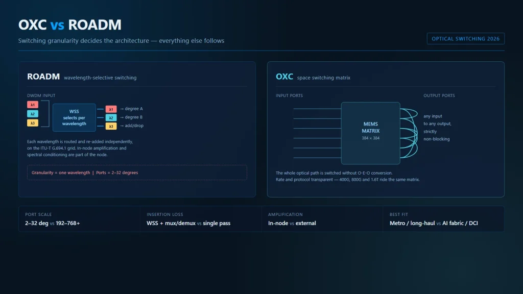
Short answer: A ROADM switches whole wavelengths, so it suits line-side transport where entire lambdas are added and dropped. An OXC switches inside the node at fibre-port granularity, which delivers wavelength, fibre and spatial switching with far higher port counts. For 2026 AI fabrics and dense metro nodes that need per-lane grooming and non-blocking growth, OXC is the better fit; for long-haul line systems and lean metro rings, ROADM remains the cheaper and better-proven choice.
Every optical network planner working on AI clusters, metro aggregation, or wholesale transport eventually faces the same fork in the road. The traffic forecast has been revised upward again, the fiber is already in the ground, and someone in the room asks the question that decides the next five years of capital spending: should the next node be a ROADM or an OXC?
The two terms are often used interchangeably in vendor presentations, and that is where trouble starts. A ROADM and an OXC solve different problems at different granularities, and picking the wrong one does not show up as a link failure. It shows up eighteen months later as stranded capacity, an exhausted optical budget, or a switching layer that cannot be reconfigured without a truck roll.
This article separates the two architectures on the dimensions that actually matter to a design review: switching granularity, port scale, blocking behavior, insertion loss, latency, power, control plane, and operational fit. It closes with a decision framework you can apply directly to a real topology, plus the deployment details that determine whether either platform performs as specified.
What a ROADM Actually Is
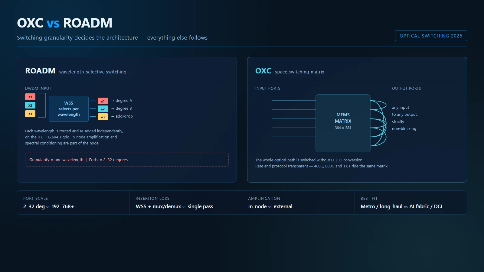
A reconfigurable optical add-drop multiplexer is a wavelength-layer node. Its job is to take a multi-wavelength DWDM signal arriving on one fiber, selectively pass some wavelengths through toward another direction, and drop the rest to local transponders. The core component is the wavelength-selective switch, which disperses the incoming spectrum and steers individual wavelength channels to chosen outputs.
Two internal architectures dominate. In a broadcast-and-select ROADM, the incoming signal is split to every WSS and each WSS selects the wavelengths it needs; the splitter introduces a fixed loss penalty that grows with degree count. In a route-and-select ROADM, a WSS sits on both the ingress and egress side, which removes the splitter loss and scales more gracefully to high degree counts. Most new metro builds use route-and-select for exactly this reason.
ROADM capability is usually described by a four-letter shorthand. Colorless means any transponder can use any wavelength on any port. Directionless means any transponder can reach any network degree. Contentionless means two transponders using the same wavelength can be added simultaneously on different degrees. Gridless means the node is not locked to a fixed channel plan and can place carriers on flexible widths. A node with all four is the most flexible — and the most expensive — ROADM you can buy.
The channel plan itself comes from the ITU-T G.694.1 frequency grid, which anchors DWDM channels on a 193.1 THz reference with spacings that start at 12.5 GHz and scale up through 25, 50, and 100 GHz. Every wavelength decision a ROADM makes is ultimately a decision about slots on that grid, which is why the grid definition matters even to engineers who never touch a WSS directly.
What an OXC Actually Is
An optical cross-connect is a space-switching matrix. Instead of selecting wavelengths on the grid, it takes an entire optical path arriving on one input port and connects it to any output port, in the optical domain, without optoelectronic conversion. The switching engine is typically a three-dimensional MEMS mirror array, a liquid-crystal-on-silicon matrix, or a planar lightwave circuit, and the port count is the defining specification.
The scale difference is the point. A metro ROADM node might present two to sixteen network degrees with a few dozen add/drop ports. A data-center OXC routinely presents 192, 384, or 768 bidirectional ports in a single chassis, and larger matrices are built by cascading stages. That is what allows an OXC to sit as the single optical hub of a fabric rather than as one node in a chain of many.
Because the signal never leaves the optical domain, an OXC is transparent to line rate and protocol. A path carrying 100G, 400G, 800G, or 1.6T rides the same matrix with no configuration change, and the matrix does not care whether the payload is Ethernet, Fibre Channel, InfiniBand, or a proprietary AI fabric protocol. For a longer treatment of the underlying principles, see our guide to optical cross-connect fundamentals.
One distinction is worth stating plainly, because it causes most of the confusion in procurement meetings: a large multi-degree ROADM and a small OXC overlap in function, but they are engineered around different bottlenecks. The ROADM is optimized for wavelength grooming along a linear or ring topology. The OXC is optimized for high-radix, any-to-any connectivity inside a confined footprint. When a vendor calls a 32-degree CDC ROADM an OXC, they are describing scale, not a different physics.
Side-by-Side Comparison
| Dimension | ROADM | OXC |
|---|---|---|
| Switching granularity | Wavelength (per ITU-T grid slot) | Whole optical path / fiber port |
| Core technology | Wavelength-selective switch (MEMS, LCOS, LC, PLC) | Space switch matrix (3D MEMS, LCOS, PLC) |
| Typical port scale | 2–32 degrees, tens of add/drop ports | 192–768+ duplex ports per chassis |
| Blocking behavior | Depends on CDC implementation | Strictly non-blocking by design |
| Insertion loss per path | Higher: WSS stages plus mux/demux plus splitter loss | Lower: single pass through the matrix |
| Rate and protocol transparency | Transparent at wavelength level | Transparent at any rate, any protocol |
| Grooming below one wavelength | Possible via transponder and OTN layer | Requires external transponder |
| Reconfiguration latency | Milliseconds at the device, seconds via controller | Milliseconds at the device, seconds via controller |
| Power per switching element | Higher: amplifiers and WSS control electronics | Lower: passive matrix, minimal control power |
| Amplification | Integrated optical amplifiers at each degree | Typically external, planned separately |
| Dominant deployment | Metro, regional, long-haul, wholesale transport | AI data centers, DCI hubs, lab and test fabrics |
| Operational maturity | Very high, two decades of deployment | High in data centers, growing in metro |
Granularity: The Decision That Cannot Be Undone
Granularity is the constraint that survives every later optimization. A ROADM can carve capacity into individual wavelengths and hand each one to a different destination, which means a single fiber pair can serve several customers, several service classes, or several protection paths at once. An OXC moves the entire path, so the unit of allocation is the whole fiber or the whole wavelength carried on it.
If your revenue model depends on selling 100G or 400G slices out of a shared spectrum, the ROADM is not optional. The moment you need per-wavelength assignment at line rate, the wavelength layer has to be addressable, and only a wavelength-selective element makes it addressable.
If your traffic model is a fixed set of very large pipes between homogeneous endpoints — GPU racks talking to GPU racks, storage pods talking to compute pods — per-wavelength slicing adds cost without adding value. You are not selling slices of a wavelength; you are moving bulk capacity between two points that need to be reconfigurable on a weekly or monthly cadence. That is the case where the OXC wins on both capital and loss budget.
Port Scale and Blocking Behavior
A ROADM’s blocking behavior is a direct consequence of how its add/drop stages are built. A colorless, directionless but non-contentionless node will refuse a second connection on the same wavelength to a different degree, even though the physical capacity exists. Contentionless add/drop stages solve this by using a dedicated switch fabric in front of the WSS, at a real cost in footprint and insertion loss. Planners who specify CDC without examining contentionless behavior often discover the limitation only during a restoration event, which is the worst possible time.
An OXC matrix is strictly non-blocking: any idle input can reach any idle output regardless of what other connections are established. That property is what makes an OXC attractive as the center of a fabric, because connection admission becomes a simple check against free ports rather than a wavelength-contention puzzle across degrees.
High-radix fabrics also change the cabling economics. A 384-port OXC in one chassis replaces several stages of leaf-spine fiber runs and the patch panels that support them. For dense physical-layer details on managing that cabling, our guide to MPO versus MTP connectors covers the polarity and density trade-offs that appear as soon as port counts climb.
Optical Budget: Where the Two Architectures Diverge Most
Insertion loss is the quiet discriminator. A ROADM path traverses a WSS on ingress, a WSS on egress, the mux and demux stages of the add/drop structure, and often a splitter if the node is broadcast-and-select. Each of those contributes loss, and the accumulated figure dictates how far the next amplifier can be pushed and what transceiver sensitivity you actually need.
An OXC path traverses one pass through the switching matrix plus connector and fiber losses. The matrix itself is typically a low-loss element because it does no spectral filtering; it simply folds light from one port to another. The practical consequence is more margin for reach, more tolerance for connector contamination and aging, and less reliance on amplification inside the node.
The trade-off is that an OXC provides no amplification and no spectral conditioning. If the span needs gain, it needs a discrete amplifier, and if the spectrum needs equalization, that function has to be placed somewhere else in the path. A ROADM bundles those functions into the node; an OXC leaves them to you. Our walkthrough of optical loss budget calculation for data center links works through the arithmetic for both cases.
Loss also compounds with connector count, which is where physical-layer discipline pays off. Every cleaning lapse and every poor endface becomes a permanent tax on the budget, and in a 384-port matrix the number of connector interfaces along a path is not trivial. The procedures in our endface cleaning and inspection guide matter more as matrices grow.
Latency, Power, and Footprint
Neither architecture performs optoelectronic conversion for the switched path, so neither adds serialization or buffering delay. Switching latency is dominated by the physical actuation mechanism — MEMS mirrors settle in milliseconds, liquid crystal cells switch in a comparable range — and by the controller’s path computation. In practice, both are fast enough that the difference rarely decides a data center design. What does decide designs is power and floor space.
A ROADM node carries amplifiers, WSS control electronics, and often a shelf of OTN or transponder equipment, so its power draw scales with degree count and channel count. An OXC matrix is largely passive; the dominant power consumers are the control electronics and the cooling needed to keep the mirrors or liquid crystal cells stable. At high port counts this becomes a material difference in rack-level power density.
Footprint follows the same logic. A ROADM-based multi-degree node with full CDC capability occupies several shelves. A single-chassis OXC concentrates the same switching function into one frame. In a colocation environment where floor space is billed per rack unit, that concentration has a direct cost consequence that is easy to understate in a feature-by-feature comparison.
Control Plane and Reconfiguration Speed
Both platforms are software-defined in 2026, and the meaningful difference is what the controller can express. A ROADM controller manipulates wavelength paths: it assigns grid slots, negotiates spectrum, and manages restoration at the wavelength layer. An OXC controller manipulates port-to-port connections, which maps more naturally onto the intent-based, topology-agnostic models that AI cluster schedulers prefer.
Reconfiguration speed at the device is not the binding constraint for either. The binding constraint is the orchestration loop: how quickly the scheduler decides a new topology is needed, how that intent reaches the controller, and how the controller validates the resulting path against the optical budget. A network that can switch in milliseconds but takes twenty minutes to decide is not a dynamically reconfigurable network.
This is where an OXC aligns well with shuffle-capable optical fabrics, because the scheduler reasons about node connectivity rather than about spectrum. It is also why ROADM deployments in metro continue to lean on established GMPLS and SDN controllers, whose wavelength semantics are already mature.
Where Each Architecture Wins
The application split is clearer than the marketing suggests. In AI data centers and dense DCI hubs, the OXC’s combination of high radix, low loss, and strict non-blocking behavior matches a traffic pattern of large homogeneous flows between pools of accelerators. For a deeper look at how those fabrics are laid out, see our analysis of infinity flex modules for CPO, OXC, and low-latency AI fabrics and the companion piece on AI data center interconnect deployment challenges.
In metro and regional transport, the ROADM remains the correct choice because the traffic is inherently heterogeneous: many endpoints, many service classes, wavelength-level service delivery, and long spans that need in-node amplification and spectral management. Our article on ROADM application for dynamic link mixing in FTTx networks illustrates how that flexibility gets used in access aggregation.
The two are not mutually exclusive. A common 2026 pattern places an OXC at the data-center or DCI hub for any-to-any reconfiguration, and hands long-haul transport to a ROADM-based line system. The OXC does what it is good at — dense, low-loss, non-blocking space switching — and the ROADM does what it is good at — wavelength grooming and amplified reach.
Deployment Considerations That Decide Success
Platform choice is the easy part. What determines whether either architecture meets its promise is the physical layer around it, and that is where data center deployments most often fall short.
Start with the fiber plant. An OXC concentrates hundreds of duplex connections into one chassis, which means the trunk cables feeding it must be measured, polarity-verified, and documented before the switch is powered on. A polarity error on a 384-port matrix is not a five-minute fix; it is a troubleshooting exercise that can consume a maintenance window. Our guide to fiber polarity methods A, B, and C and the companion piece on MPO and MTP trunk cable selection cover the conventions that prevent this class of failure.
Next, plan the transceiver layer honestly. An OXC is transparent, so it will happily pass a marginal signal. That transparency cuts both ways: it means the matrix will not hide a bad link, and it means you need real measurements rather than assumptions. Rate transitions matter too — an 800G lane count is not a small step up from 400G in terms of loss tolerance, as our 800G optical interconnect guide explains.
Then consider where the optics are going. Co-packaged optics and linear pluggable designs change the loss budget by removing DSP from the module, which makes every decibel in the path more valuable. That shift strengthens the case for low-loss switching in the middle of the fabric; our overview of CPO market trends and the LPO deployment guide set out the implications for switch and interconnect design.
Finally, stage the migration. Replacing a wavelength-layer node with a space-switching matrix is not a like-for-like swap. Cabling, documentation, monitoring hooks, and the controller’s northbound interface all change. A staged approach — new fabric first, legacy wavelength services migrated after the optical budget has been verified in production — is the only reliable path. The wider trajectory of these transitions is covered in our piece on six evolution paths for next-generation optical transport.
A Decision Framework You Can Apply Today
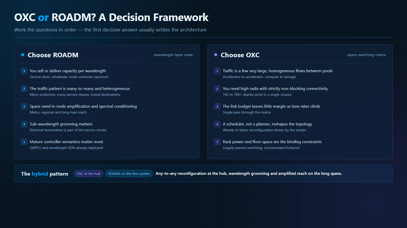
Work through these questions in order. The first one that produces a decisive answer usually settles the architecture.
- Do you sell capacity per wavelength? If yes, you need wavelength addressability: ROADM.
- Is the traffic pattern many-to-many with heterogeneous endpoints? If yes, wavelength grooming and in-node amplification matter: ROADM.
- Is the traffic pattern a small number of very large homogeneous flows between pools? If yes, radix and loss dominate: OXC.
- Does the link budget leave less than roughly six decibels of margin? If yes, the lower insertion loss of a space matrix is worth serious weight.
- Will the topology need to change weekly or faster, driven by a scheduler rather than a planner? If yes, port-level programmability is the better abstraction: OXC.
- Do you need amplification and spectral conditioning inside the node? If yes, a ROADM bundles it; an OXC will require discrete amplifiers in the path.
- Is floor space or rack power the binding constraint? If yes, single-chassis concentration favors the OXC.
Any design that answers yes to both question one and question three is not confused — it is a hybrid network, and it should be specified as one from the start rather than assembled by accident.
Frequently Asked Questions
Is an OXC simply a very large ROADM?
Not quite. A high-degree ROADM and a small OXC overlap in port count, but the ROADM selects wavelengths on the ITU grid while the OXC switches entire optical paths through a space matrix. The ROADM’s value is spectral selectivity; the OXC’s value is radix and non-blocking connectivity. Calling a 32-degree CDC ROADM an OXC describes its scale, not its function.
Can an OXC replace a ROADM in long-haul transport?
Rarely on its own. Long-haul spans need in-line amplification and per-channel spectral management, which a ROADM node bundles and a passive matrix does not. An OXC can serve as a reconfiguration hub between line systems, but the wavelength layer still has to exist somewhere. Most long-haul designs keep the ROADM and add the OXC only at junction points.
Which architecture handles sub-wavelength grooming?
Neither does it inside the optical layer. A ROADM enables grooming only when a transponder or OTN switch terminates the wavelength and reshuffles it electrically. An OXC is fully transparent and cannot touch the contents of a path at all. If sub-rate grooming is a requirement, plan for the electrical layer explicitly.
Which is better for an AI data center fabric?
For most AI cluster designs in 2026, the OXC is the better fit, for three reasons: hundreds of ports in one chassis, strict non-blocking behavior that simplifies connection admission, and low insertion loss that preserves margin as lane rates move to 800G and beyond. The exception is a facility that also delivers wavelength services to external customers, where a ROADM layer is still needed.
Does an OXC need transponders?
Not for switching, but yes for any function that requires electrical processing: rate conversion, sub-wavelength multiplexing, performance monitoring at the frame level, or encryption. A pure OXC fabric moves light and nothing else, which is precisely why it is fast, low-power, and rate-agnostic.
How do the two compare on insertion loss?
A ROADM path accumulates loss from WSS stages, mux and demux structures, and splitter stages in broadcast-and-select designs. An OXC path makes a single pass through the matrix. The matrix is the lower-loss element, but the OXC node omits amplification, so the comparison must be made on the complete end-to-end path rather than on the switching component alone.
Which one should a greenfield metro build choose?
A route-and-select ROADM with colorless, directionless, and contentionless add/drop is the default for greenfield metro, because service delivery is wavelength-based and spans need amplification. Add OXC capability at hubs where any-to-any reconfiguration between line systems is expected, rather than replacing the wavelength layer wholesale.
What standards should the design reference?
Use the ITU-T G.694.1 frequency grid for any wavelength plan, IEEE 802.3 for the Ethernet rates that ride on it, and the Open Compute Project's optical specifications when specifying data-center hardware that must interoperate across vendors. Anchoring the design to published references keeps vendor conversations honest.
The Bottom Line
ROADM and OXC are not competing answers to the same question. The ROADM answers “which wavelength goes where” and brings amplification and spectral management with it. The OXC answers “which port connects to which port” and brings radix, transparency, and low loss. Metro transport, wholesale, and any network that sells capacity per wavelength will keep its ROADM layer. AI fabrics, dense DCI hubs, and any topology that a scheduler needs to reshape on demand will increasingly center on the OXC.
The designs that fail are the ones that pick a platform before answering the granularity and loss questions. Answer those two first, and the architecture usually selects itself.
References: ITU-T G.694.1 spectral grids for WDM applications; IEEE 802.3 Ethernet standards; Open Compute Project optical specifications.